
When Midday PV Meets Fleet Demand
At 1 PM on a sunny Tuesday, the commercial plant room carries two distinct sounds: the steady operation of a solar inverter at maximum yield and the sharper pull of contactors as fleet vans connect to their chargers. The contactors typically close somewhere around two to four seconds after plug detection. In that short interval, an exporting site can become a substantial importer.
The fleet charging plan had been built around midday photovoltaic generation. Vehicles would return, connect while the array was productive, and absorb energy that might otherwise pass into the grid. That principle was sound, but the main incomer still governed what the site could carry at any instant.
The Incomer Sets the Boundary
A charger cannot assume that full inverter output remains available for vehicles. Offices, workshops, ventilation and other building loads consume part of the generation before any surplus reaches the supply tails. When several vans latch in close succession, their combined demand can also rise faster than solar output can respond.
The immediate design question is therefore precise: how much EV charging load can be admitted without taking the site beyond its Agreed Supply Capacity?
A supply-capacity upgrade may resolve that constraint, although the required programme can be too slow for an operational fleet. In this case, the existing capacity was retained and active load control was placed ahead of the charging demand. The controller had to reconcile volatile generation, changing building consumption and vehicle demand before the main incomer approached its limit.
Midday Collision: Maximum PV yield does not establish charger headroom. The usable allowance is the surplus remaining after the building load has been accounted for at the incoming supply point.
Measuring Surplus and Controlling the Incomer
Standard plug-and-play charging treats the charge point as an available load once a vehicle connects. Subject to its configured rating and the vehicle request, the charger can begin drawing from the supply without following the site's solar balance. That behaviour is simple, but it can place a significant new demand on existing commercial infrastructure.
How Solar Matching Uses Export
Solar-matching mode bases charge current on measured surplus. Export monitoring at the supply tails identifies the energy left after the building has consumed its share of PV generation. The charge point management system then uses that residual value as its charging allowance.
- The solar array generates on the AC side of the installation.
- Existing building loads consume part of that output.
- The grid current transformer measures the remaining import or export at the incoming tails.
- The management system converts measured surplus into an available EV charging current.
- The charger increases or reduces demand as the measured balance changes.
Inverter telemetry alone cannot provide the same control reference. It reports solar production, while the grid current transformer sees the residual position after building consumption. A productive array can therefore coexist with little or no genuine surplus.
Dynamic Control Against the ASC
Solar matching manages how much PV surplus the vehicles use. Dynamic load management provides a second boundary by checking charging demand against the site's Agreed Supply Capacity. If the wider building load rises, the system throttles the EV load before the main incomer approaches its rating.
This arrangement is commonly required when a substantial EV load is added without reinforcing the incoming commercial supply. It supports Distribution Network Operator conditions and the addition-of-load requirements in BS 7671:2018+A2:2022, provided that the control measurement represents the correct supply boundary.
Supply Boundary: The control case applies only where the export CT sits on the tails that define the Agreed Supply Capacity. A CT on a downstream EV or PV board cannot establish total site headroom.
Placing Grid and Solar CTs Where Readings Count
Two clamps perform two separate jobs. The grid CT belongs on the incoming tails, where it can measure the site's net relationship with the grid. The solar CT belongs on the PV AC conductors, where it can measure inverter output. Treating the clamps as interchangeable undermines the export calculation.
Installation Sequence
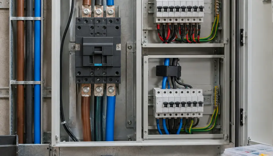
- Identify the ASC measurement point. Locate the incoming tails that carry the site's combined building, PV and EV position. This is the grid CT location.
- Fit the grid CT on the incoming tails. Keep the measurement at the supply boundary rather than moving it to the EV board incomer.
- Locate the PV AC conductors. Fit the separate solar CT there so the management system can distinguish generation from net grid flow.
- Set both arrows toward the load. The directional markings establish the expected sign for import, export and generation.
- Prove arrow direction and polarity. Confirm the readings before the charge point management system is permitted to close a contactor.
Why the EV Board Gives the Wrong Picture
A grid CT placed on the EV board incomer sees charger current alone. It misses the wider building demand and the PV contribution, so the controller cannot calculate either true solar surplus or remaining headroom at the main incomer.
The error can look plausible on a dashboard. Charger demand appears to be measured, values change when a vehicle connects, and the charge point responds. Yet the central arithmetic remains incomplete because the measurement excludes the loads that define the supply constraint.
Polarity Before Permission
An inverted grid CT reverses the sign of the reading. Export can appear as import, and import can appear as export. Under solar matching, that reversal can produce the exact behaviour the design was intended to prevent: the charger draws from the grid while the array exports.
Polarity should therefore be treated as a commissioning gate. The system must demonstrate that an exporting condition is displayed as export and that a rising site load reduces the available charging allowance. Only then should contactor operation be enabled.
Arrow Check: Grid and solar CT arrows point load-ward. A neat installation with reversed polarity still supplies unusable control data.
Setting Solar Start and Site Current Ceilings
Configuration begins after CT polarity has been proven. Parameter entry should reflect vehicle wake behaviour and the site's ASC rather than the maximum hardware rating printed on the charger.
Set the Solar Start Threshold
A typical single-phase EV onboard charger needs approximately 1.4 kW before it will accept a charge. Setting the minimum export threshold at that level gives the vehicle a usable starting condition. It also prevents repeated attempts to begin charging when only a thin margin of export is available.
- Select the solar-matching operating mode in the charge point management system.
- Confirm that the grid and solar CT channels display the intended direction.
- Enter 1.4 kW as the minimum export required to initiate a single-phase charging session.
- Observe whether the connected vehicle wakes and accepts current when the threshold is reached.
- Confirm that charging reduces when measured surplus falls.
This threshold controls the start of a solar-led session. It does not replace the hard current ceiling needed to protect the incoming supply.
Write the Hard Limit Against Headroom
The dynamic current limit should be referenced to the Agreed Supply Capacity and the headroom left by the rest of the site. When building demand rises, the management system reduces EV current first. When headroom returns, charging can increase within the configured boundary.

The supervised parameter session on the live incomer requires a dedicated observation period. That time should include observing real measurements, checking charger response and confirming that the hard limit remains active while solar matching changes the requested current.
- Solar threshold: decides when measured export is sufficient to wake the vehicle.
- Solar-matching request: follows the surplus available at the incoming tails.
- Dynamic current limit: prevents EV demand from consuming capacity reserved by the site's ASC boundary.
These settings form a hierarchy. The charger may have enough solar surplus to increase output, yet the dynamic limit can still hold it back because the building load has reduced total site headroom.
Proving Load Response Before Handover
A charger powering up proves only basic operation. Handover should wait until the installation has followed live changes in generation and protected the incoming supply while doing so.
Run a Live Solar Response Test
The final observation window should cover a sustained period. A cloud-edge drop provides a useful reduction in PV output, followed by recovery as generation rises again. The test team can then watch the dashboard and charger response move with the measured supply condition.
- Begin with the inverter generating and a vehicle connected.
- Confirm that the dashboard shows the expected solar output and grid direction.
- Observe the charger during a reduction in generation.
- Verify that charging demand falls before the incomer approaches its configured boundary.
- Observe recovery and confirm that charging increases as genuine surplus returns.
- Introduce a site-load change where available and check that the dynamic limit retains priority.
The important evidence is coordinated movement: the CT reading changes, the management system recalculates the allowance, and the charger follows. A static screenshot cannot demonstrate that sequence.
Leave the Facility Manager a Usable Record
The handover pack should explain the reporting dashboard, the visible effect of solar matching and the circumstances in which charging will throttle. It should also record the control settings, CT locations and the load behaviour observed during commissioning. Where scheme documentation applies, installers should check the current Workplace Charging Scheme technical requirements.
The facility manager should be able to distinguish a controlled reduction from a fault. Lower charging power during high building demand can show that the system is protecting the agreed supply boundary exactly as configured.
A single 22 kW three-phase charger draws roughly 32 A per phase; on a 100 A per phase commercial supply, one connected vehicle consumes nearly a third of the available capacity.